
 Logo:
Logo:  Areas Served:
  with Python — Tutorial")
Natural Language Processing (NLP) with Python — Tutorial
Last Updated on October 21, 2021 by Editorial Team
Author(s): Pratik Shukla, Roberto Iriondo
Natural Language Processing, Scholarly, Tutorial
Tutorial on the basics of natural language processing (NLP) with sample code implementation in Python
In this article, we explore the basics of natural language processing (NLP) with code examples. We dive into the natural language toolkit (NLTK) library to present how it can be useful for natural language processing related-tasks. Afterward, we will discuss the basics of other Natural Language Processing libraries and other essential methods for NLP, along with their respective coding sample implementations in Python.
📚 Resources: Google Colab Implementation | GitHub Repository 📚
Table of Contents:
- What is Natural Language Processing?
- Applications of NLP
- Understanding Natural Language Processing (NLP)
- Rule-based NLP vs. Statistical NLP
- Components of Natural Language Processing (NLP)
- Current challenges in NLP
- Easy to Use NLP Libraries
- Exploring Features of NLTK
- Word Cloud
- Stemming
- Lemmatization
- Part-of-Speech (PoS) tagging
- Chunking
- Chinking
- Named Entity Recognition (NER)
- WordNet
- Bag of Words
- TF-IDF
What is Natural Language Processing?
Computers and machines are great at working with tabular data or spreadsheets. However, as human beings generally communicate in words and sentences, not in the form of tables. Much information that humans speak or write is unstructured. So it is not very clear for computers to interpret such. In natural language processing (NLP), the goal is to make computers understand the unstructured text and retrieve meaningful pieces of information from it. Natural language Processing (NLP) is a subfield of artificial intelligence, in which its depth involves the interactions between computers and humans.
Applications of NLP:
- Machine Translation.
- Speech Recognition.
- Sentiment Analysis.
- Question Answering.
- Summarization of Text.
- Chatbot.
- Intelligent Systems.
- Text Classifications.
- Character Recognition.
- Spell Checking.
- Spam Detection.
- Autocomplete.
- Named Entity Recognition.
- Predictive Typing.
Understanding Natural Language Processing (NLP):
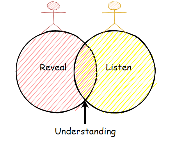
We, as humans, perform natural language processing (NLP) considerably well, but even then, we are not perfect. We often misunderstand one thing for another, and we often interpret the same sentences or words differently.
For instance, consider the following sentence, we will try to understand its interpretation in many different ways:
Example 1:

These are some interpretations of the sentence shown above.
- There is a man on the hill, and I watched him with my telescope.
- There is a man on the hill, and he has a telescope.
- I’m on a hill, and I saw a man using my telescope.
- I’m on a hill, and I saw a man who has a telescope.
- There is a man on a hill, and I saw him something with my telescope.
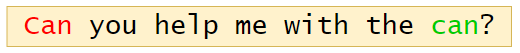
Example 2:
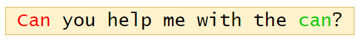
In the sentence above, we can see that there are two “can” words, but both of them have different meanings. Here the first “can” word is used for question formation. The second “can” word at the end of the sentence is used to represent a container that holds food or liquid.
Hence, from the examples above, we can see that language processing is not “deterministic” (the same language has the same interpretations), and something suitable to one person might not be suitable to another. Therefore, Natural Language Processing (NLP) has a non-deterministic approach. In other words, Natural Language Processing can be used to create a new intelligent system that can understand how humans understand and interpret language in different situations.
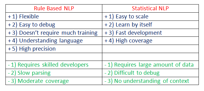
Rule-based NLP vs. Statistical NLP:
Natural Language Processing is separated in two different approaches:
Rule-based Natural Language Processing:
It uses common sense reasoning for processing tasks. For instance, the freezing temperature can lead to death, or hot coffee can burn people’s skin, along with other common sense reasoning tasks. However, this process can take much time, and it requires manual effort.
Statistical Natural Language Processing:
It uses large amounts of data and tries to derive conclusions from it. Statistical NLP uses machine learning algorithms to train NLP models. After successful training on large amounts of data, the trained model will have positive outcomes with deduction.
Comparison:
Components of Natural Language Processing (NLP):
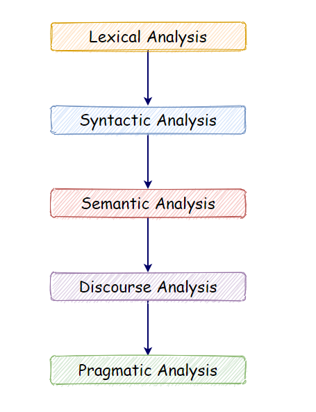
a. Lexical Analysis:
With lexical analysis, we divide a whole chunk of text into paragraphs, sentences, and words. It involves identifying and analyzing words’ structure.
b. Syntactic Analysis:
Syntactic analysis involves the analysis of words in a sentence for grammar and arranging words in a manner that shows the relationship among the words. For instance, the sentence “The shop goes to the house” does not pass.
c. Semantic Analysis:
Semantic analysis draws the exact meaning for the words, and it analyzes the text meaningfulness. Sentences such as “hot ice-cream” do not pass.
d. Disclosure Integration:
Disclosure integration takes into account the context of the text. It considers the meaning of the sentence before it ends. For example: “He works at Google.” In this sentence, “he” must be referenced in the sentence before it.
e. Pragmatic Analysis:
Pragmatic analysis deals with overall communication and interpretation of language. It deals with deriving meaningful use of language in various situations.
📚 Check out an overview of machine learning algorithms for beginners with code examples in Python. 📚
Current challenges in NLP:
- Breaking sentences into tokens.
- Tagging parts of speech (POS).
- Building an appropriate vocabulary.
- Linking the components of a created vocabulary.
- Understanding the context.
- Extracting semantic meaning.
- Named Entity Recognition (NER).
- Transforming unstructured data into structured data.
- Ambiguity in speech.
Easy to use NLP libraries:
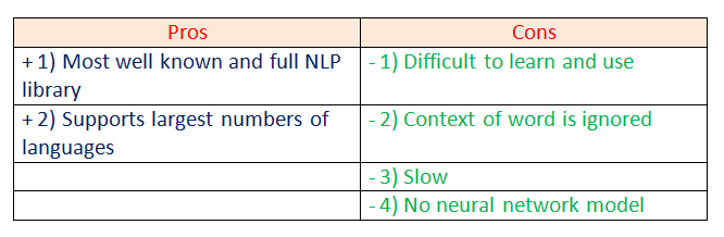
a. NLTK (Natural Language Toolkit):
The NLTK Python framework is generally used as an education and research tool. It’s not usually used on production applications. However, it can be used to build exciting programs due to its ease of use.
Features:
- Tokenization.
- Part Of Speech tagging (POS).
- Named Entity Recognition (NER).
- Classification.
- Sentiment analysis.
- Packages of chatbots.
Use-cases:
- Recommendation systems.
- Sentiment analysis.
- Building chatbots.
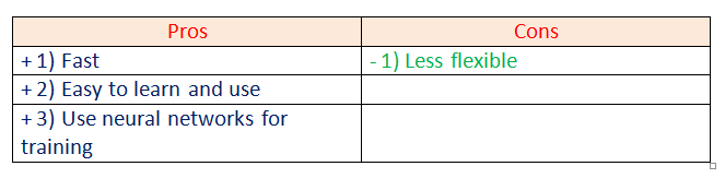
b. spaCy:
spaCy is an open-source natural language processing Python library designed to be fast and production-ready. spaCy focuses on providing software for production usage.
Features:
- Tokenization.
- Part Of Speech tagging (POS).
- Named Entity Recognition (NER).
- Classification.
- Sentiment analysis.
- Dependency parsing.
- Word vectors.
Use-cases:
- Autocomplete and autocorrect.
- Analyzing reviews.
- Summarization.
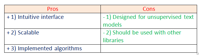
c. Gensim:
Gensim is an NLP Python framework generally used in topic modeling and similarity detection. It is not a general-purpose NLP library, but it handles tasks assigned to it very well.
Features:
- Latent semantic analysis.
- Non-negative matrix factorization.
- TF-IDF.
Use-cases:
- Converting documents to vectors.
- Finding text similarity.
- Text summarization.
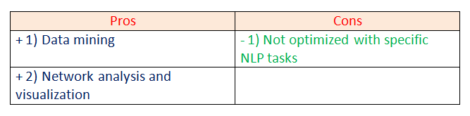
d. Pattern:
Pattern is an NLP Python framework with straightforward syntax. It’s a powerful tool for scientific and non-scientific tasks. It is highly valuable to students.
Features:
- Tokenization.
- Part of Speech tagging.
- Named entity recognition.
- Parsing.
- Sentiment analysis.
Use-cases:
- Spelling correction.
- Search engine optimization.
- Sentiment analysis.
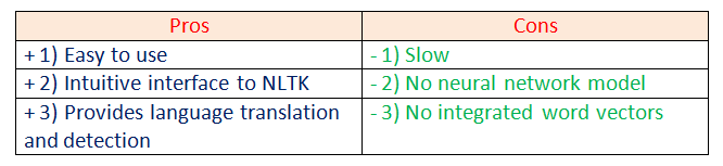
e. TextBlob:
TextBlob is a Python library designed for processing textual data.
Features:
- Part-of-Speech tagging.
- Noun phrase extraction.
- Sentiment analysis.
- Classification.
- Language translation.
- Parsing.
- Wordnet integration.
Use-cases:
- Sentiment Analysis.
- Spelling Correction.
- Translation and Language Detection.
For this tutorial, we are going to focus more on the NLTK library. Let’s dig deeper into natural language processing by making some examples.
Exploring Features of NLTK:
a. Open the text file for processing:
First, we are going to open and read the file which we want to analyze.
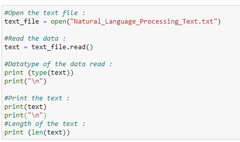
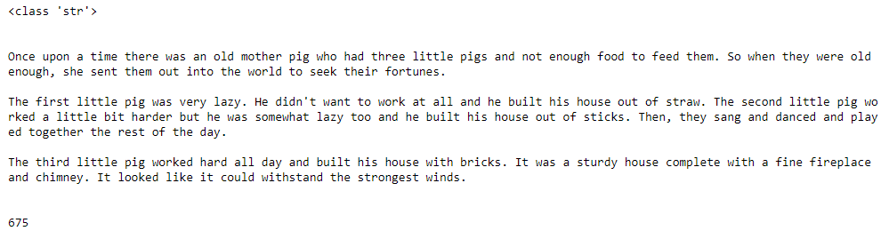
Next, notice that the data type of the text file read is a String. The number of characters in our text file is 675.
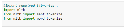
b. Import required libraries:
For various data processing cases in NLP, we need to import some libraries. In this case, we are going to use NLTK for Natural Language Processing. We will use it to perform various operations on the text.
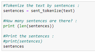
c. Sentence tokenizing:
By tokenizing the text with sent_tokenize( ), we can get the text as sentences.
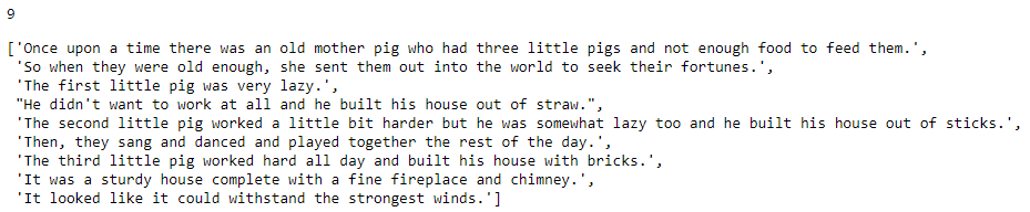
In the example above, we can see the entire text of our data is represented as sentences and also notice that the total number of sentences here is 9.
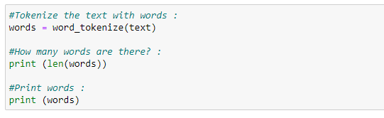
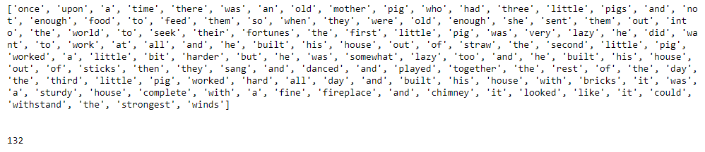
d. Word tokenizing:
By tokenizing the text with word_tokenize( ), we can get the text as words.
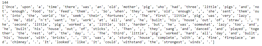
Next, we can see the entire text of our data is represented as words and also notice that the total number of words here is 144.
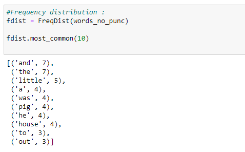
e. Find the frequency distribution:
Let’s find out the frequency of words in our text.
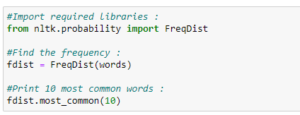
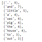
Notice that the most used words are punctuation marks and stopwords. We will have to remove such words to analyze the actual text.
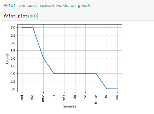
f. Plot the frequency graph:
Let’s plot a graph to visualize the word distribution in our text.
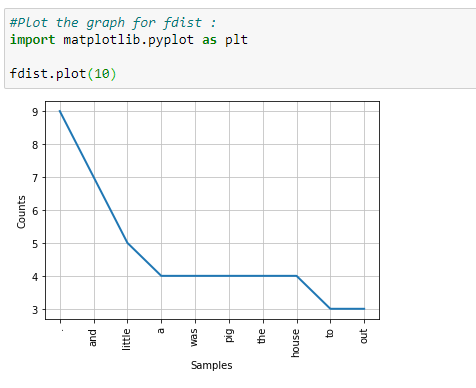
In the graph above, notice that a period “.” is used nine times in our text. Analytically speaking, punctuation marks are not that important for natural language processing. Therefore, in the next step, we will be removing such punctuation marks.
g. Remove punctuation marks:
Next, we are going to remove the punctuation marks as they are not very useful for us. We are going to use isalpha( ) method to separate the punctuation marks from the actual text. Also, we are going to make a new list called words_no_punc, which will store the words in lower case but exclude the punctuation marks.
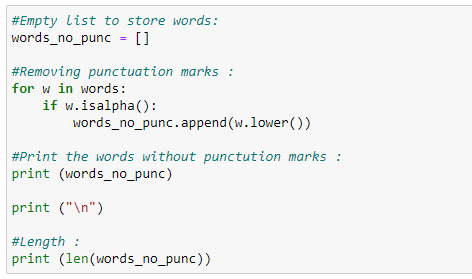
As shown above, all the punctuation marks from our text are excluded. These can also cross-check with the number of words.
h. Plotting graph without punctuation marks:
Notice that we still have many words that are not very useful in the analysis of our text file sample, such as “and,” “but,” “so,” and others. Next, we need to remove coordinating conjunctions.
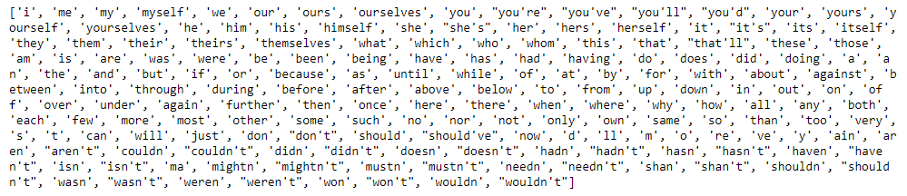
i. List of stopwords:
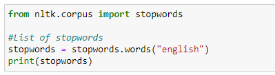
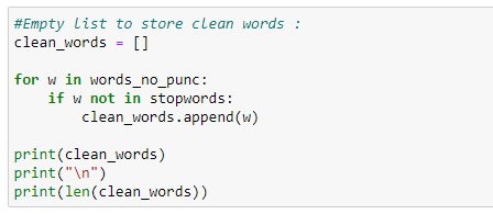
j. Removing stopwords:
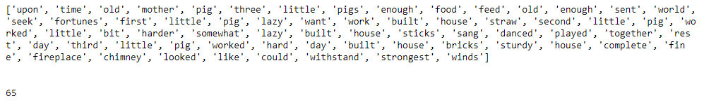
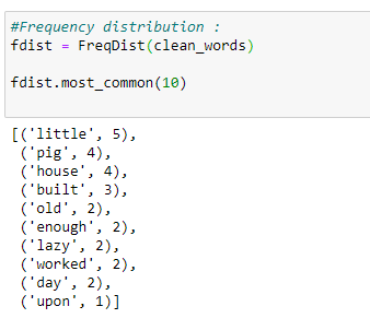
k. Final frequency distribution:
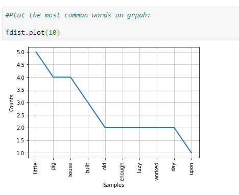
As shown above, the final graph has many useful words that help us understand what our sample data is about, showing how essential it is to perform data cleaning on NLP.
Next, we will cover various topics in NLP with coding examples.
Word Cloud:
Word Cloud is a data visualization technique. In which words from a given text display on the main chart. In this technique, more frequent or essential words display in a larger and bolder font, while less frequent or essential words display in smaller or thinner fonts. It is a beneficial technique in NLP that gives us a glance at what text should be analyzed.
Properties:
- font_path: It specifies the path for the fonts we want to use.
- width: It specifies the width of the canvas.
- height: It specifies the height of the canvas.
- min_font_size: It specifies the smallest font size to use.
- max_font_size: It specifies the largest font size to use.
- font_step: It specifies the step size for the font.
- max_words: It specifies the maximum number of words on the word cloud.
- stopwords: Our program will eliminate these words.
- background_color: It specifies the background color for canvas.
- normalize_plurals: It removes the trailing “s” from words.
Read the full documentation on WordCloud.
Word Cloud Python Implementation:
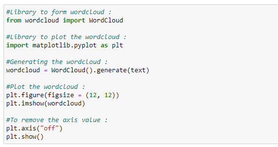
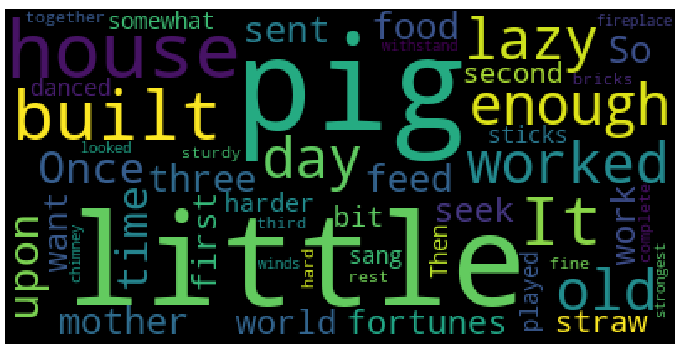
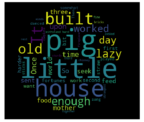
As shown in the graph above, the most frequent words display in larger fonts. The word cloud can be displayed in any shape or image.
For instance: In this case, we are going to use the following circle image, but we can use any shape or any image.

Word Cloud Python Implementation:
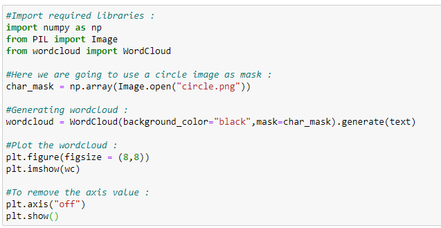
As shown above, the word cloud is in the shape of a circle. As we mentioned before, we can use any shape or image to form a word cloud.
Word CloudAdvantages:
- They are fast.
- They are engaging.
- They are simple to understand.
- They are casual and visually appealing.
Word Cloud Disadvantages:
- They are non-perfect for non-clean data.
- They lack the context of words.
Stemming:
We use Stemming to normalize words. In English and many other languages, a single word can take multiple forms depending upon context used. For instance, the verb “study” can take many forms like “studies,” “studying,” “studied,” and others, depending on its context. When we tokenize words, an interpreter considers these input words as different words even though their underlying meaning is the same. Moreover, as we know that NLP is about analyzing the meaning of content, to resolve this problem, we use stemming.
Stemming normalizes the word by truncating the word to its stem word. For example, the words “studies,” “studied,” “studying” will be reduced to “studi,” making all these word forms to refer to only one token. Notice that stemming may not give us a dictionary, grammatical word for a particular set of words.
Let’s take an example:
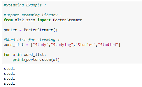
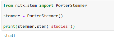
a. Porter’s Stemmer Example 1:
In the code snippet below, we show that all the words truncate to their stem words. However, notice that the stemmed word is not a dictionary word.
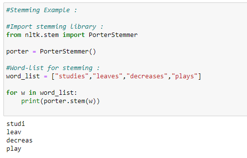
b. Porter’s Stemmer Example 2:
In the code snippet below, many of the words after stemming did not end up being a recognizable dictionary word.
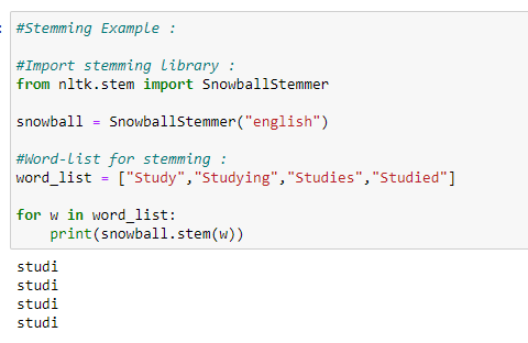
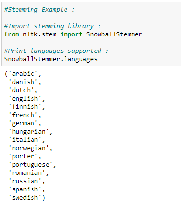
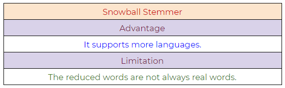
c. SnowballStemmer:
SnowballStemmer generates the same output as porter stemmer, but it supports many more languages.
d. Languages supported by snowball stemmer:
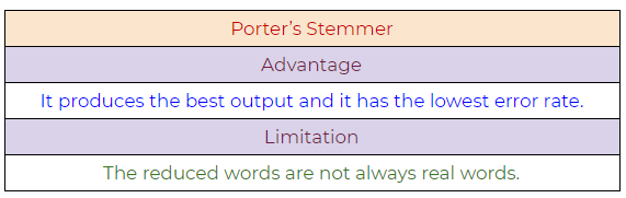
Various Stemming Algorithms:
a. Porter’s Stemmer:
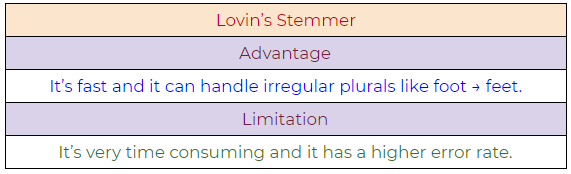
b. Lovin’s Stemmer:
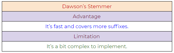
c. Dawson’s Stemmer:
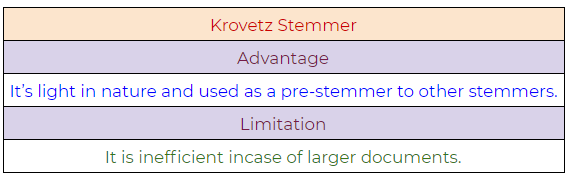
d. Krovetz Stemmer:
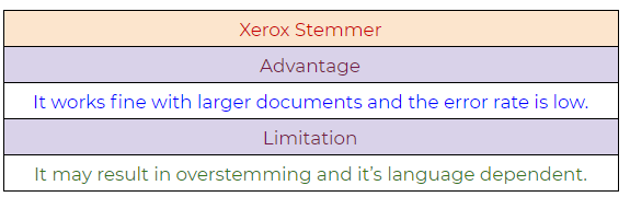
e. Xerox Stemmer:
f. Snowball Stemmer:
📚 Check out our tutorial on neural networks from scratch with Python code and math in detail.📚
Lemmatization:
Lemmatization tries to achieve a similar base “stem” for a word. However, what makes it different is that it finds the dictionary word instead of truncating the original word. Stemming does not consider the context of the word. That is why it generates results faster, but it is less accurate than lemmatization.
If accuracy is not the project’s final goal, then stemming is an appropriate approach. If higher accuracy is crucial and the project is not on a tight deadline, then the best option is amortization (Lemmatization has a lower processing speed, compared to stemming).
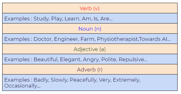
Lemmatization takes into account Part Of Speech (POS) values. Also, lemmatization may generate different outputs for different values of POS. We generally have four choices for POS:
Difference between Stemmer and Lemmatizer:
a. Stemming:
Notice how on stemming, the word “studies” gets truncated to “studi.”
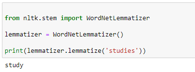
b. Lemmatizing:
During lemmatization, the word “studies” displays its dictionary word “study.”
Python Implementation:
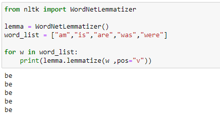
a. A basic example demonstrating how a lemmatizer works
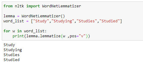
In the following example, we are taking the PoS tag as “verb,” and when we apply the lemmatization rules, it gives us dictionary words instead of truncating the original word:
b. Lemmatizer with default PoS value
The default value of PoS in lemmatization is a noun(n). In the following example, we can see that it’s generating dictionary words:
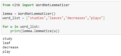
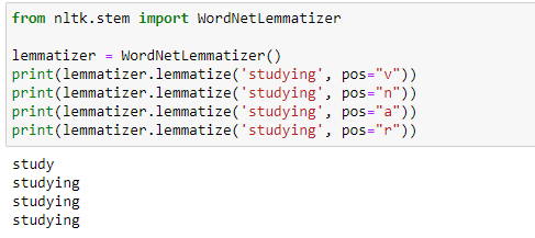
c. Another example demonstrating the power of lemmatizer
d. Lemmatizer with different POS values
Part of Speech Tagging (PoS tagging):
Why do we need Part of Speech (POS)?
Parts of speech(PoS) tagging is crucial for syntactic and semantic analysis. Therefore, for something like the sentence above, the word “can” has several semantic meanings. The first “can” is used for question formation. The second “can” at the end of the sentence is used to represent a container. The first “can” is a verb, and the second “can” is a noun. Giving the word a specific meaning allows the program to handle it correctly in both semantic and syntactic analysis.
Below, please find a list of Part of Speech (PoS) tags with their respective examples:
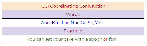
1. CC: Coordinating Conjunction
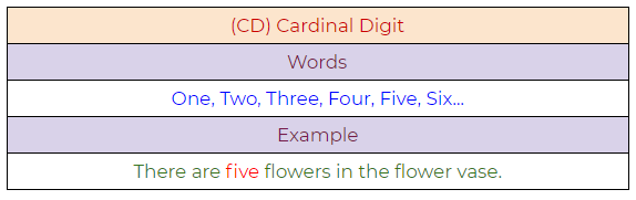
2. CD: Cardinal Digit
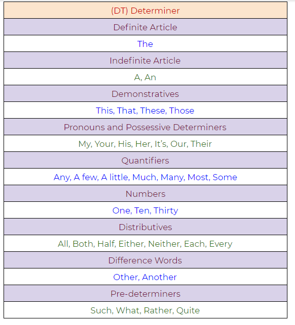
3. DT: Determiner
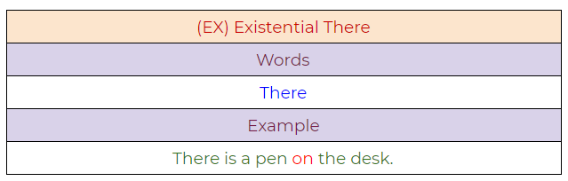
4. EX: Existential There
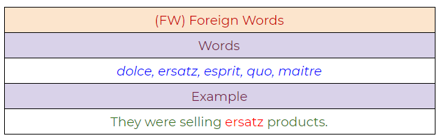
5. FW: Foreign Word
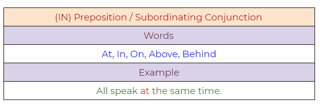
6. IN: Preposition / Subordinating Conjunction
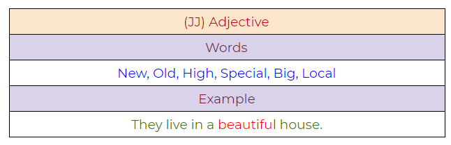
7. JJ: Adjective
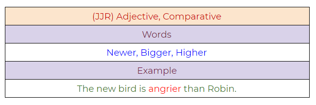
8. JJR: Adjective, Comparative
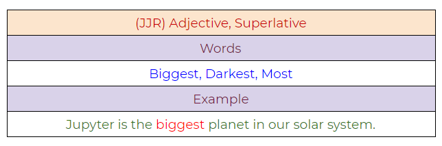
9. JJS: Adjective, Superlative
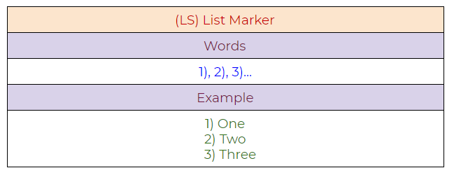
10. LS: List Marker
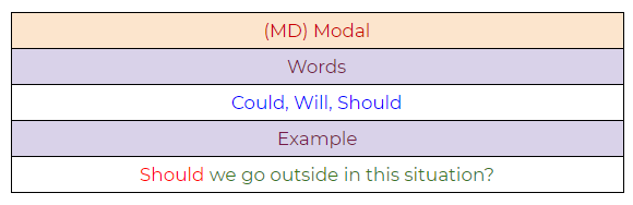
11. MD: Modal
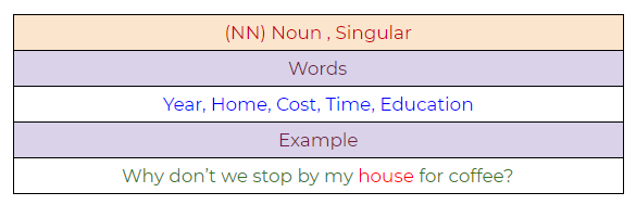
12. NN: Noun, Singular
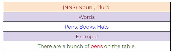
13. NNS: Noun, Plural
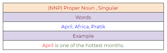
14. NNP: Proper Noun, Singular
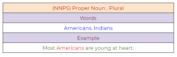
15. NNPS: Proper Noun, Plural
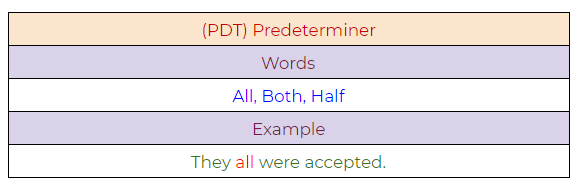
16. PDT: Predeterminer
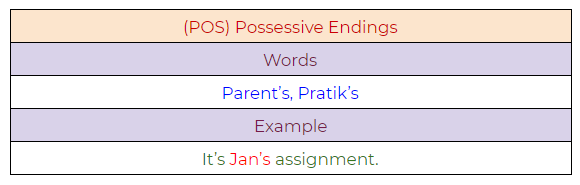
17. POS: Possessive Endings
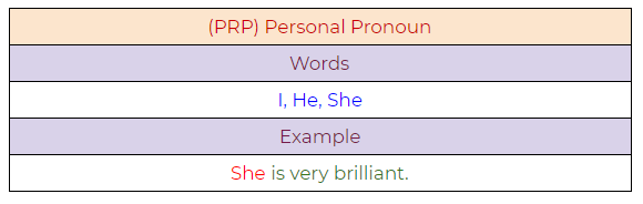
18. PRP: Personal Pronoun
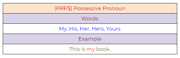
19. PRP$: Possessive Pronoun
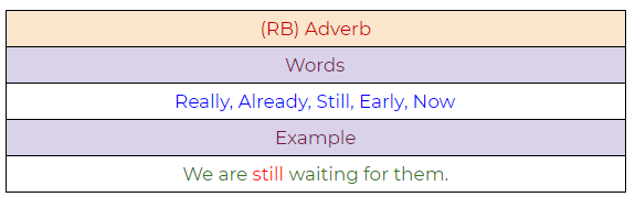
20. RB: Adverb
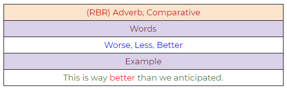
21. RBR: Adverb, Comparative
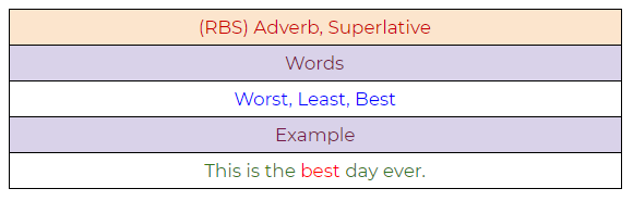
22. RBS: Adverb, Superlative
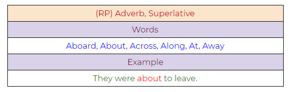
23. RP: Particle
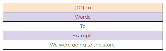
24. TO: To
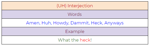
25. UH: Interjection
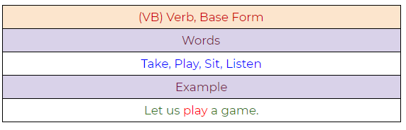
26. VB: Verb, Base Form
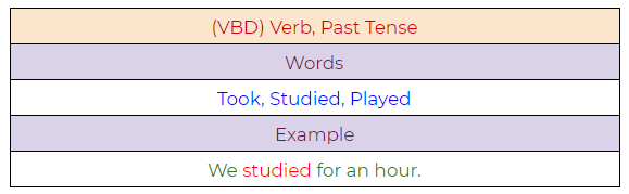
27. VBD: Verb, Past Tense
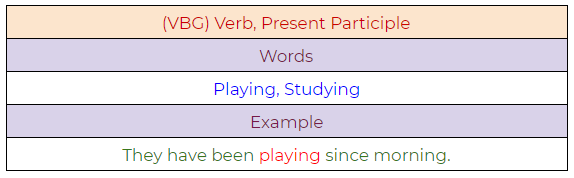
28. VBG: Verb, Present Participle
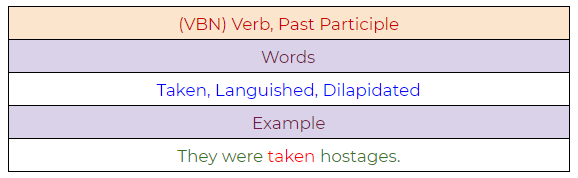
29. VBN: Verb, Past Participle
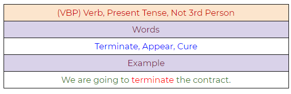
30. VBP: Verb, Present Tense, Not Third Person Singular
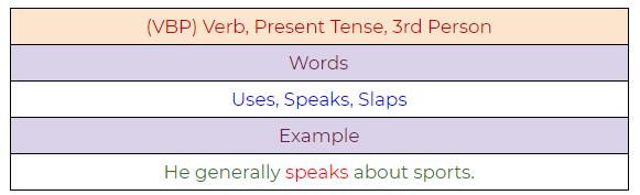
31. VBZ: Verb, Present Tense, Third Person Singular
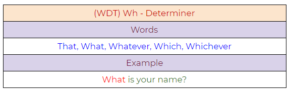
32. WDT: Wh — Determiner
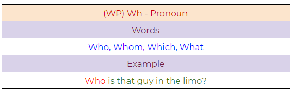
33. WP: Wh — Pronoun
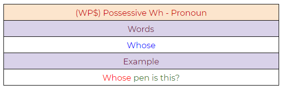
34. WP$ : Possessive Wh — Pronoun
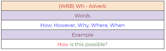
35. WRB: Wh — Adverb
Python Implementation:
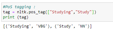
a. A simple example demonstrating PoS tagging.
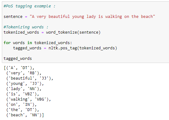
b. A full example demonstrating the use of PoS tagging.
Chunking:
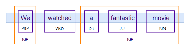
Chunking means to extract meaningful phrases from unstructured text. By tokenizing a book into words, it’s sometimes hard to infer meaningful information. It works on top of Part of Speech(PoS) tagging. Chunking takes PoS tags as input and provides chunks as output. Chunking literally means a group of words, which breaks simple text into phrases that are more meaningful than individual words.
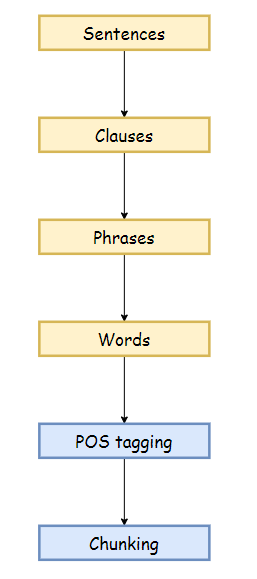
Before working with an example, we need to know what phrases are? Meaningful groups of words are called phrases. There are five significant categories of phrases.
- Noun Phrases (NP).
- Verb Phrases (VP).
- Adjective Phrases (ADJP).
- Adverb Phrases (ADVP).
- Prepositional Phrases (PP).
Phrase structure rules:
- S(Sentence) → NP VP.
- NP → {Determiner, Noun, Pronoun, Proper name}.
- VP → V (NP)(PP)(Adverb).
- PP → Pronoun (NP).
- AP → Adjective (PP).
Example:
Python Implementation:
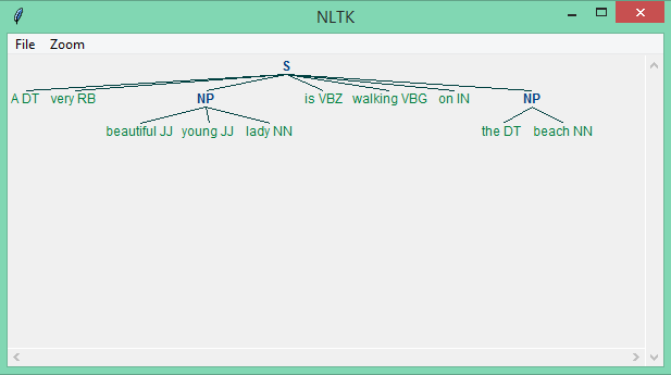
In the following example, we will extract a noun phrase from the text. Before extracting it, we need to define what kind of noun phrase we are looking for, or in other words, we have to set the grammar for a noun phrase. In this case, we define a noun phrase by an optional determiner followed by adjectives and nouns. Then we can define other rules to extract some other phrases. Next, we are going to use RegexpParser( ) to parse the grammar. Notice that we can also visualize the text with the .draw( ) function.
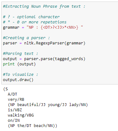
In this example, we can see that we have successfully extracted the noun phrase from the text.
Chinking:
Chinking excludes a part from our chunk. There are certain situations where we need to exclude a part of the text from the whole text or chunk. In complex extractions, it is possible that chunking can output unuseful data. In such case scenarios, we can use chinking to exclude some parts from that chunked text.
In the following example, we are going to take the whole string as a chunk, and then we are going to exclude adjectives from it by using chinking. We generally use chinking when we have a lot of unuseful data even after chunking. Hence, by using this method, we can easily set that apart, also to write chinking grammar, we have to use inverted curly braces, i.e.:
} write chinking grammar here {
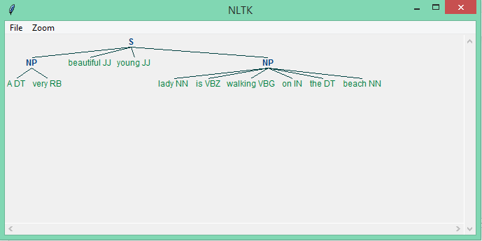
Python Implementation:
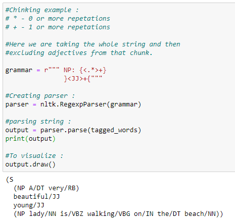
From the example above, we can see that adjectives separate from the other text.
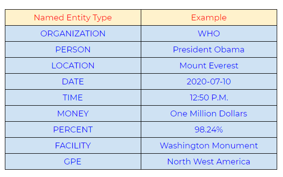
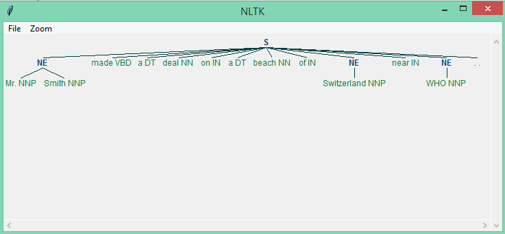
Named Entity Recognition (NER):
Named entity recognition can automatically scan entire articles and pull out some fundamental entities like people, organizations, places, date, time, money, and GPE discussed in them.
Use-Cases:
- Content classification for news channels.
- Summarizing resumes.
- Optimizing search engine algorithms.
- Recommendation systems.
- Customer support.
Commonly used types of named entity:
Python Implementation:
There are two options :
1. binary = True
When the binary value is True, then it will only show whether a particular entity is named entity or not. It will not show any further details on it.
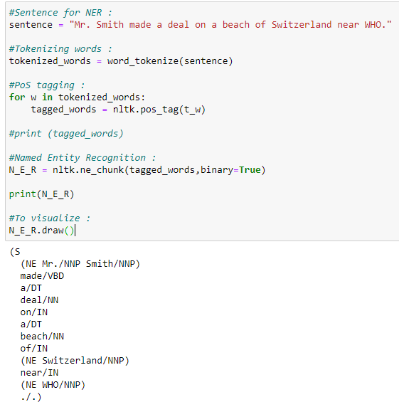
Our graph does not show what type of named entity it is. It only shows whether a particular word is named entity or not.
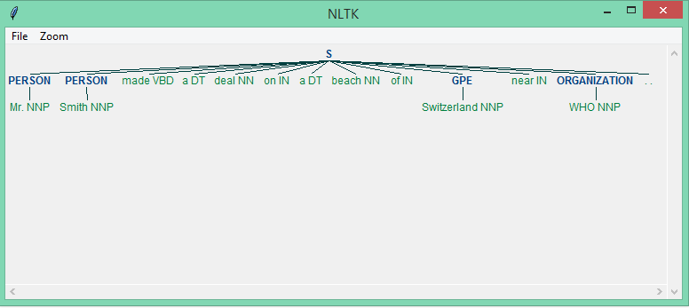
2. binary = False
When the binary value equals False, it shows in detail the type of named entities.
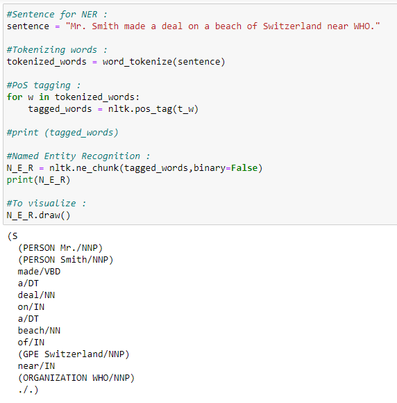
Our graph now shows what type of named entity it is.
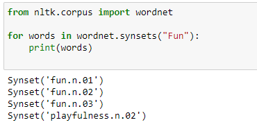
WordNet:
Wordnet is a lexical database for the English language. Wordnet is a part of the NLTK corpus. We can use Wordnet to find meanings of words, synonyms, antonyms, and many other words.
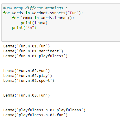
a. We can check how many different definitions of a word are available in Wordnet.
b. We can also check the meaning of those different definitions.
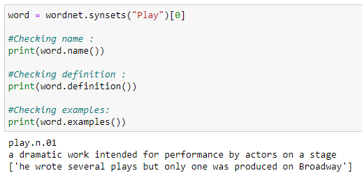
c. All details for a word.
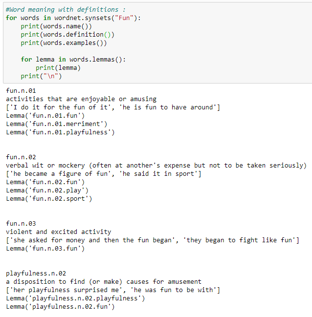
d. All details for all meanings of a word.
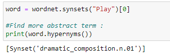
e. Hypernyms: Hypernyms gives us a more abstract term for a word.
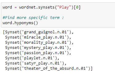
f. Hyponyms: Hyponyms gives us a more specific term for a word.
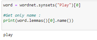
g. Get a name only.
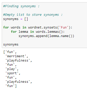
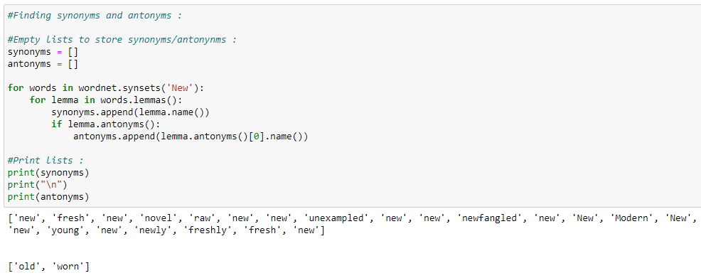
h. Synonyms.
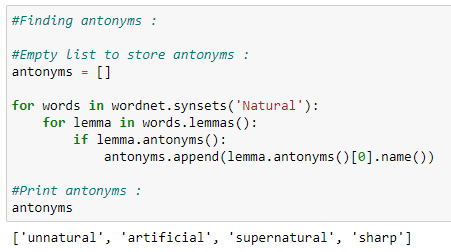
i. Antonyms.
j. Synonyms and antonyms.
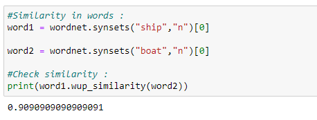
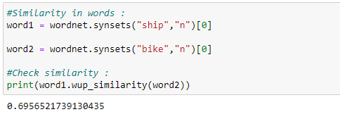
k. Finding the similarity between words.
Bag of Words:
What is the Bag-of-Words method?
It is a method of extracting essential features from row text so that we can use it for machine learning models. We call it “Bag” of words because we discard the order of occurrences of words. A bag of words model converts the raw text into words, and it also counts the frequency for the words in the text. In summary, a bag of words is a collection of words that represent a sentence along with the word count where the order of occurrences is not relevant.
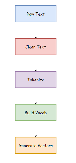
- Raw Text: This is the original text on which we want to perform analysis.
- Clean Text: Since our raw text contains some unnecessary data like punctuation marks and stopwords, so we need to clean up our text. Clean text is the text after removing such words.
- Tokenize: Tokenization represents the sentence as a group of tokens or words.
- Building Vocab: It contains total words used in the text after removing unnecessary data.
- Generate Vocab: It contains the words along with their frequencies in the sentences.
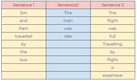
For instance:
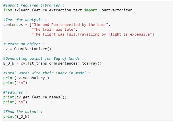
Sentences:
- Jim and Pam traveled by bus.
- The train was late.
- The flight was full. Traveling by flight is expensive.
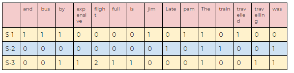
a. Creating a basic structure:
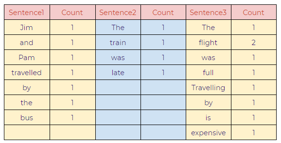
b. Words with frequencies:
c. Combining all the words:
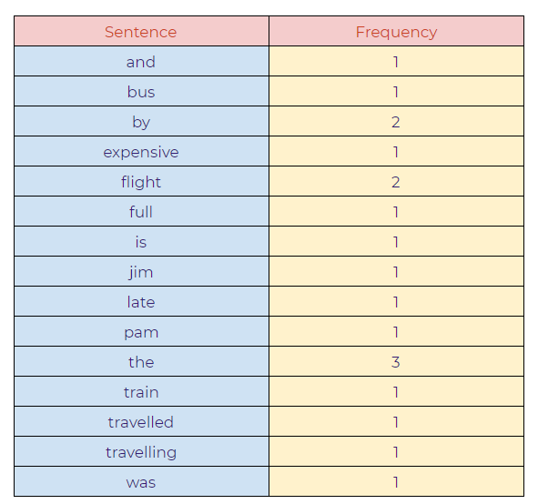
d. Final model:
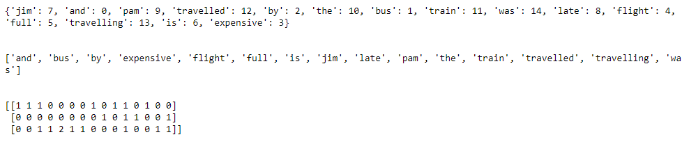
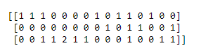
Python Implementation:
Applications:
- Natural language processing.
- Information retrieval from documents.
- Classifications of documents.
Limitations:
- Semantic meaning: It does not consider the semantic meaning of a word. It ignores the context in which the word is used.
- Vector size: For large documents, the vector size increase, which may result in higher computational time.
- Preprocessing: In preprocessing, we need to perform data cleansing before using it.
TF-IDF
TF-IDF stands for Term Frequency — Inverse Document Frequency, which is a scoring measure generally used in information retrieval (IR) and summarization. The TF-IDF score shows how important or relevant a term is in a given document.
The intuition behind TF and IDF:
If a particular word appears multiple times in a document, then it might have higher importance than the other words that appear fewer times (TF). At the same time, if a particular word appears many times in a document, but it is also present many times in some other documents, then maybe that word is frequent, so we cannot assign much importance to it. (IDF). For instance, we have a database of thousands of dog descriptions, and the user wants to search for “a cute dog” from our database. The job of our search engine would be to display the closest response to the user query. How would a search engine do that? The search engine will possibly use TF-IDF to calculate the score for all of our descriptions, and the result with the higher score will be displayed as a response to the user. Now, this is the case when there is no exact match for the user’s query. If there is an exact match for the user query, then that result will be displayed first. Then, let’s suppose there are four descriptions available in our database.
- The furry dog.
- A cute doggo.
- A big dog.
- The lovely doggo.
Notice that the first description contains 2 out of 3 words from our user query, and the second description contains 1 word from the query. The third description also contains 1 word, and the forth description contains no words from the user query. As we can sense that the closest answer to our query will be description number two, as it contains the essential word “cute” from the user’s query, this is how TF-IDF calculates the value.
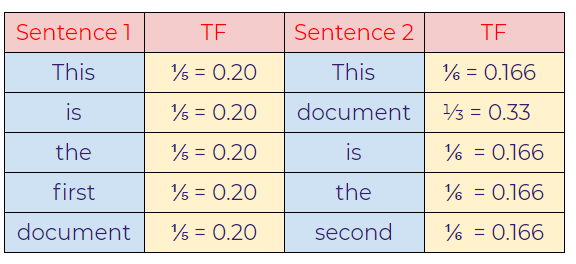
Notice that the term frequency values are the same for all of the sentences since none of the words in any sentences repeat in the same sentence. So, in this case, the value of TF will not be instrumental. Next, we are going to use IDF values to get the closest answer to the query. Notice that the word dog or doggo can appear in many many documents. Therefore, the IDF value is going to be very low. Eventually, the TF-IDF value will also be lower. However, if we check the word “cute” in the dog descriptions, then it will come up relatively fewer times, so it increases the TF-IDF value. So the word “cute” has more discriminative power than “dog” or “doggo.” Then, our search engine will find the descriptions that have the word “cute” in it, and in the end, that is what the user was looking for.
Simply put, the higher the TF*IDF score, the rarer or unique or valuable the term and vice versa.
Now we are going to take a straightforward example and understand TF-IDF in more detail.
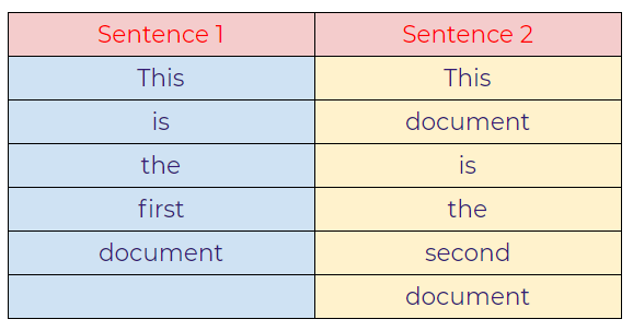
Example:
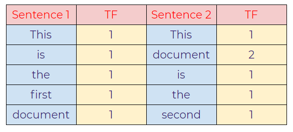
Sentence 1: This is the first document.
Sentence 2: This document is the second document.
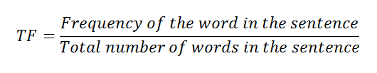
TF: Term Frequency
a. Represent the words of the sentences in the table.
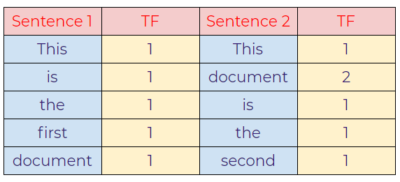
b. Displaying the frequency of words.
c. Calculating TF using a formula.

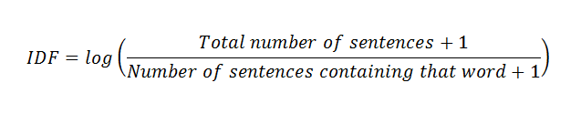
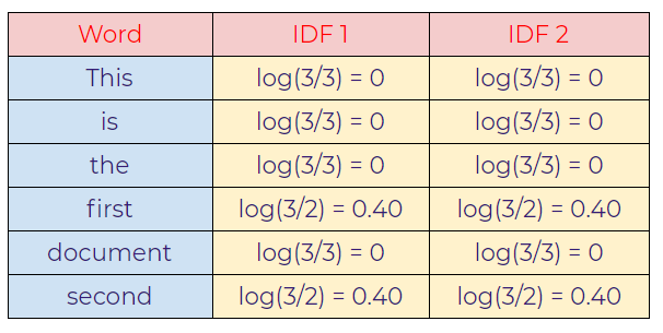
IDF: Inverse Document Frequency
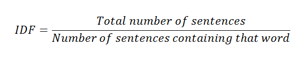
d. Calculating IDF values from the formula.
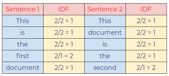
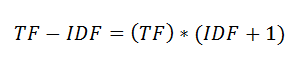
e. Calculating TF-IDF.
TF-IDF is the multiplication of TF*IDF.
In this case, notice that the import words that discriminate both the sentences are “first” in sentence-1 and “second” in sentence-2 as we can see, those words have a relatively higher value than other words.
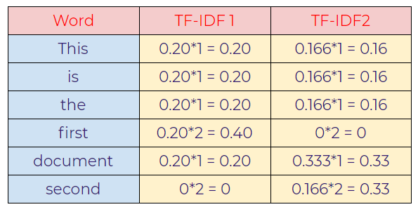
However, there any many variations for smoothing out the values for large documents. The most common variation is to use a log value for TF-IDF. Let’s calculate the TF-IDF value again by using the new IDF value.
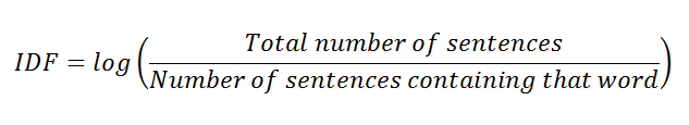
f. Calculating IDF value using log.
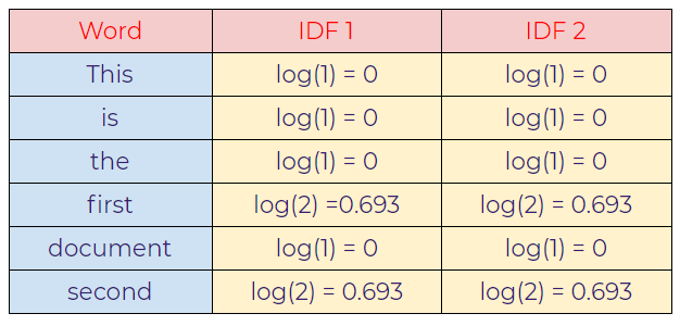
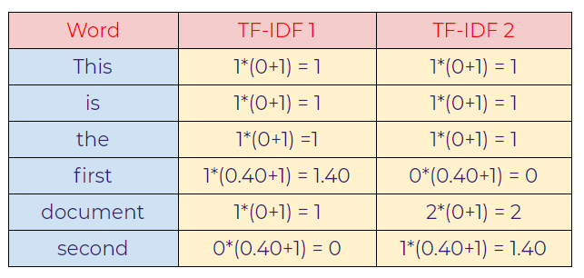
g. Calculating TF-IDF.
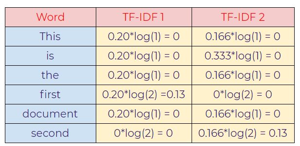
As seen above, “first” and “second” values are important words that help us to distinguish between those two sentences.
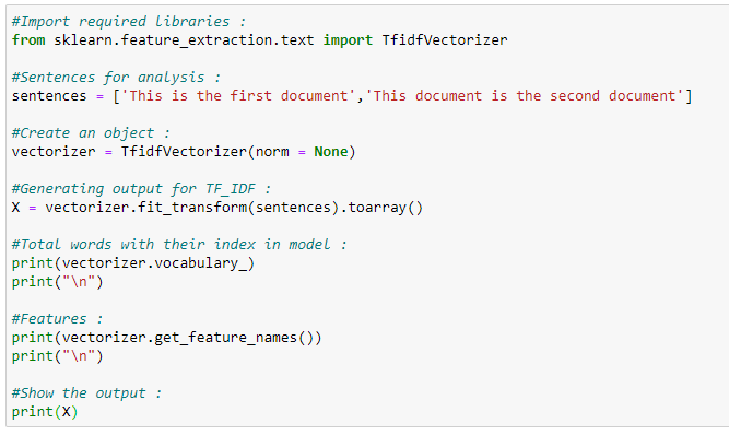
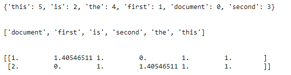
Now that we saw the basics of TF-IDF. Next, we are going to use the sklearn library to implement TF-IDF in Python. A different formula calculates the actual output from our program. First, we will see an overview of our calculations and formulas, and then we will implement it in Python.
Actual Calculations:
a. Term Frequency (TF):
b. Inverse Document Frequency (IDF):
c. Calculating final TF-IDF values:
Python Implementation:
Conclusion:
These are some of the basics for the exciting field of natural language processing (NLP). We hope you enjoyed reading this article and learned something new. Any suggestions or feedback is crucial to continue to improve. Please let us know in the comments if you have any.
DISCLAIMER: The views expressed in this article are those of the author(s) and do not represent the views of Carnegie Mellon University, nor other companies (directly or indirectly) associated with the author(s). These writings do not intend to be final products, yet rather a reflection of current thinking, along with being a catalyst for discussion and improvement.
Published via Towards AI
Citation
For attribution in academic contexts, please cite this work as:
Shukla, et al., “Natural Language Processing (NLP) with Python — Tutorial”, Towards AI, 2020
BibTex citation:
@article{pratik_iriondo_2020,
 title={Natural Language Processing (NLP) with Python — Tutorial},
 url={https://towardsai.net/nlp-tutorial-with-python},
 journal={Towards AI},
 publisher={Towards AI Co.},
 author={Pratik, Shukla and Iriondo, Roberto},
 year={2020},
 month={Jul}
}
References:
[1] The example text was gathered from American Literature, https://americanliterature.com/
[2] Natural Language Toolkit, https://www.nltk.org/
[3] TF-IDF, KDnuggets, https://www.kdnuggets.com/2018/08/wtf-tf-idf.html
Resources:
Related posts


Comments (4)
Feedback ↓
Popular posts

 for 2021")


Updates

Recent Posts


Avremee
very well explanations, thank you
Shivakumar Kokkula
Superb content
Hemalatha Abothula
good
javed khan
great explanation